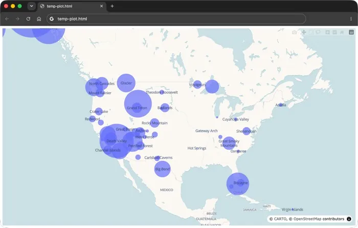
Plot National Parks!:
Read in the Dataset with Pandas:
- To acquire a deeper understanding, we can read in a dataset using Pandas of national park locations in the US. (the national-parks.csv data file is available on Canvas).
- On line 7 we can sample the data at the tail end of the dataframe using the tail method.
python
1import plotly.graph_objs as go
2import plotly.offline as offline
3import pandas as pd
4
5df = pd.read_csv('national-parks.csv')
6df.tail()
7print(df.tail())
Output:
1    Latitude  Longitude                Park  State(s) ...       Area    Visitors
256     43.57    -103.48           Wind Cave        SD ...   33970.84      656397
357     61.00    -142.00  Wrangell–St. Elias        AK ... 8323146.00       79450
458     44.60    -110.50         Yellowstone  WY,MT,ID ... 2219790.00     4115000
559     37.83    -119.50            Yosemite        CA ...  761747.50     4009436
660     37.30    -113.05                Zion        UT ...  147237.02     4320033
Obtain the list of latitudes and longitudes:
- On lines 9 and 10 below, we can extract the latitude and longitude information for these parks using the Pandas dataframe.
Set a scaling factor:
- On line 11, we can manually apply a scaling factor of 500 to increase the scale value and reduce the size of the markers
Define the trace:
- Line 13 instantiates the Scattermap object. We pass in the lats/longs as separate arrays as before on lines 14 and 15.
- The size of every marker that represents a park shows the size, representing the area in acres by manually dividing the area data by the scale factor we set up in the above.
Define the layout:
- To setup a layout of our visualization, we can instantiate the go.Layout() class on line 21.
python
8# ---snip ---
9latitudes = df["Latitude"]
10longitudes = df["Longitude"]
11scale = 500
12
13trace = go.Scattermap(
14    lat = latitudes,
15    lon = longitudes,
16    mode = "markers+text",
17    text = df["Park"],
18    marker = dict(size = df["Area"] / scale, sizemode = "area"),
19)
20
21layout = go.Layout(
22    map=dict(
23        style = "carto-voyager",
24        center = dict(lat=39.5, lon=-98.35),
25        zoom = 3
26    ),
27    margin={"r":0,"t":0,"l":0,"b":0})
28
29data = [trace]
30fig = dict(data = data, layout = layout)
31offline.plot(fig)
Output: